 1
 2
 3
 4
 5
 6
 7
 8
 9
10
11
12
13
14
15
16
17
18
19
20
21
22
23
24
25
26
27
28
29
30
31
32
33
34
35
36
37
38
39
40
41
42
43
44
45
46
47
48
49
50
51
52
53
54
55
56
57
58
59
60
61
62
63
64
65
66
67
68
69
70
71
72
73
74
75
76
77
78
79
80
81
82
83
84
85
86
| from keras.datasets import mnist
from keras.layers import Input, Dense
from keras.models import Model
import numpy as np
import matplotlib.pyplot as plt
EPOCHS = 50
BATCH_SIZE = 256
def train(x_train, x_test):
input_img = Input(shape=(784,))
# 三个编码层,将数据从 784 维向量编码为 128、64、32 维向量
encoded = Dense(units=128, activation='relu')(input_img)
encoded = Dense(units=64, activation='relu')(encoded)
encoded = Dense(units=32, activation='relu')(encoded)
# 三个解码层,将数据从 32 维向量解码成 64、128、784 维向量
decoded = Dense(units=64, activation='relu')(encoded)
decoded = Dense(units=128, activation='relu')(decoded)
decoded = Dense(units=784, activation='sigmoid')(decoded)
autoencoder = Model(input_img, decoded)
encoder = Model(input_img, encoded)
autoencoder.summary()
encoder.summary()
autoencoder.compile(optimizer='adam', loss='binary_crossentropy', metrics=['accuracy'])
autoencoder.fit(x_train, x_train,
epochs=EPOCHS,
batch_size=BATCH_SIZE,
shuffle=True,
validation_data=(x_test, x_test))
return encoder, autoencoder
def plot(encoded_imgs, decoded_imgs):
plt.figure(figsize=(40, 4))
for i in range(10):
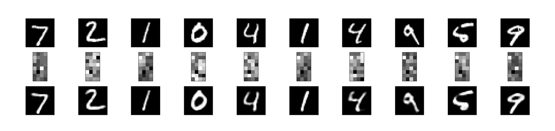
# 展示原始输入图像
ax = plt.subplot(3, 20, i + 1)
plt.imshow(x_test[i].reshape(28, 28))
plt.gray()
ax.get_xaxis().set_visible(False)
ax.get_yaxis().set_visible(False)
# 展示编码后的图像
ax = plt.subplot(3, 20, i + 1 + 20)
plt.imshow(encoded_imgs[i].reshape(8, 4))
plt.gray()
ax.get_xaxis().set_visible(False)
ax.get_yaxis().set_visible(False)
# 展示解码后的输入图像
ax = plt.subplot(3, 20, 2 * 20 + i + 1)
plt.imshow(decoded_imgs[i].reshape(28, 28))
plt.gray()
ax.get_xaxis().set_visible(False)
ax.get_yaxis().set_visible(False)
plt.show()
if __name__ == '__main__':
# 加载数据,训练数据 60000 条,测试数据 10000 条,数据灰度值 [0, 255]
(x_train, _), (x_test, _) = mnist.load_data()
# 正则化数据,将灰度值区间转换为 [0, 1]
x_train = x_train.astype('float32') / 255
x_test = x_test.astype('float32') / 255
# 将数据集从二维 (28, 28) 矩阵转换为长度为维度是 784 的向量
x_train = x_train.reshape(len(x_train), np.prod(x_train.shape[1:]))
x_test = x_test.reshape(len(x_test), np.prod(x_test.shape[1:]))
print(x_train.shape)
print(x_test.shape)
# 训练数据
encoder, autoencoder = train(x_train, x_test)
# 获取编码后和解码后的图像
encoded_imgs = encoder.predict(x_test)
decoded_imgs = autoencoder.predict(x_test)
# 绘制图像
plot(encoded_imgs, decoded_imgs)
|